5.13.3 Cox regression

Due to the characteristics of data sets designed for survival analyses, traditional regression methods are not used, but specialised survival models, of which Cox is one of the most common.

In short, survival models such as Cox are used to estimate which variables affect the hazard risk the most. In contrast to standard regression analysis which estimates effects of explanatory variables on a response variable where all variables are measured at a given time, the focus in Cox models is on estimating the effect of explanatory variables on relative hazard risk linked to a specific event (death, illness, disability, unemployment etc) which is measured over time. More specifically, the hazard rate is estimated given by h(t|x), i.e. the hazard rate as a function of t (time) and x (set of explanatory variables).

Cox can be seen as a more formalised method for comparing the effects of explanatory variables on survival time/hazard risk compared to Kaplan-Meier where survival rate curves are generated and shifts in these are studied through splitting according to different characteristics given by categorical variables.

The Cox proportional hazard model is given by the following formula:

 

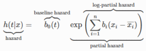
Note that the time component is only in the first part of the expression above: $b_0(t)$. This is called "baseline hazard" and is a time-dependent base component that is scaled up or down based on the second term in which the explanatory variables are included.

After you have your data set ready for survival analysis, cf. section above, you can run a Cox regression by using the command cox where you first enter the variable that measures "event" and then the variable that measures "time" (the order is important). Note that data that are adapted to other forms of survival analysis, such as Kaplan-Meier, are also compatible with Cox analysis.

Examples:

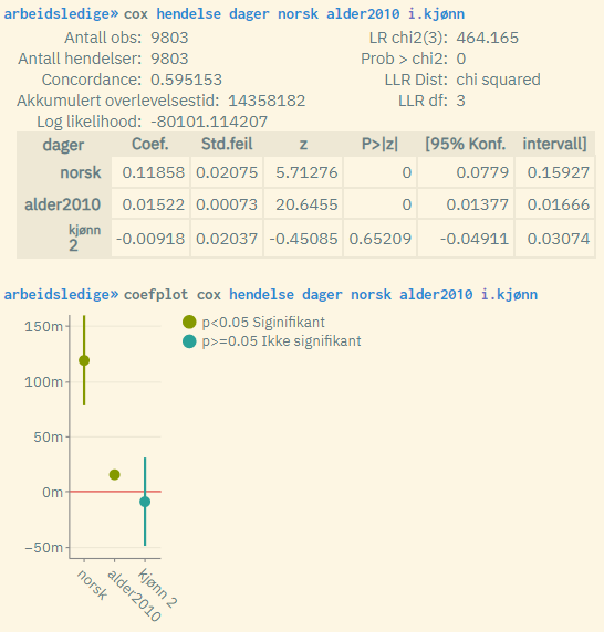
Typical result (default):

Note: "hendelse" = event, "dager" = days, "norsk" = norwegian, "alder2010" = age per 2010, "kjønn" = gender

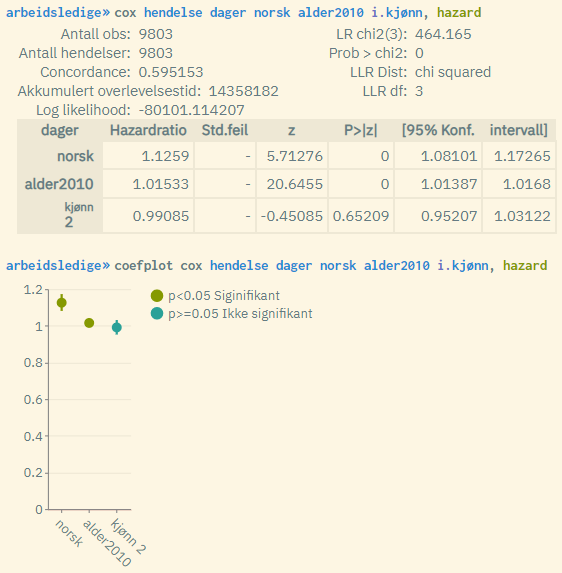
Typical result when using the hazard rate option:

Note: "hendelse" = event, "dager" = days, "norsk" = norwegian, "alder2010" = age per 2010, "kjønn" = gender

INTERPRETATION OF RESULTS

• The top example shows the default display with coefficient estimates. These should be interpreted in the traditional way. Positive coefficient values ​​mean a positive correlation between the relevant variable and hazard risk, and an implicit negative effect on survival time. Negative values ​​mean the opposite. Zero value means no correlation.

• The bottom example shows estimated hazard rates instead of coefficients. These show the rate-wise change in risk for a one-unit increase in the variable in question, and must be interpreted in a different way. The zero point that suggests no correlation is here the value 1. Values ​​above 1 mean a positive effect on risk (implicitly negative effect on survival time), and vice versa for values ​​below 1.

• Note: Positive effect on risk (i.e. negative effect on survival time) corresponds to a steeper Kaplan-Meier survival rate curve (compared to the reference group).

• The command coefplot can be used in conjunction with cox for graphical display of the estimates, as in the examples above.

• The numbers in the main table should be interpreted in the same way as for normal regressions, e.g. regress.

• The overall model measurement parameters at the top:

  • "Antall obs" = Number of observations: Number of observations included in the analysis population (= number of units/individuals in the case of regular cross-sectional data sets)

  • "Antall hendelser" = Number of events: The number of events summed over the analysis population (= the sum of the dummy variable that measures the event measured over the analysis population).

  • Concordance (C-index): An alternative to LR chi2() as a measure of explanatory power. C-index is based on compilations of actual versus predicted values ​​for all units, and the value is calculated from the proportion of matching pairs of values divided by the number of possible pairs in total. 0 is bad, 1 is best. Values ​​should be above 0.5.

  • "Akkumulert overlevelsestid" = Cumulative survival time: The sum of the variable that measures time measured across all units in the population.

  • Log likelihood: Measure of explanatory power for the model. Possible values ​​are from minus infinity to infinity. The higher the value, the better the model. But not an intuitive measurement. Instead, use "LR chi2" / "Prob > chi2" or C-index to assess whether the model is good.

  • LR chi2(): Value from chi-square test

  • "Prob > chi2": P-value for chi-square test. Low values ​​are good. Used to assess whether the model is good or bad. The value should be below 0.2.

• Baseline estimation is based on the Breslow method

 $\rhd$ Example: How to prepare data for survival analysis, amongst others Cox analyses